Abstract
We present a decision-quality pipeline for selecting operating points in zero-knowledge (ZK) systems under two competing objectives: leakage resistance and implementation cost. Using NSGA-II with SBX crossover, self-adaptive Gaussian mutation, and a stagnation-aware kick, we recover a well-spread Pareto frontier and a principled knee configuration. The leakage objective uses a linear-probe \(R^2\) on transcript features as a conservative attacker model; the cost objective is a monotone proxy for runtime/footprint suitable for later calibration with measured prover/verify metrics. From the recorded run, we quantify end-to-end changes, explain the geometry of the search surface, and provide guidance for operational deployment.
Problem Statement
Picking ZK parameters \(\theta=(a,b,c)\) that simultaneously minimize transcript leakage and resource usage is inherently multi-objective. We make this explicit by optimizing \(L(\theta)\) (leakage) and \(C(\theta)\) (cost) jointly: \( \min_{\theta\in\mathcal D} \ (L(\theta), C(\theta)) \). The outcome is a set of non-dominated solutions (the Pareto frontier). We then select a robust default via a knee that balances normalized objectives.
Leakage metric. Linear-probe \(R^2\) on transcript features (↓ better).
Cost metric. Smooth proxy \(C(\theta)=w_t T(\theta)+w_m M(\theta)+w_o O(\theta)\) (↓ better).
Code, Assumptions, and Test Protocol
Assumed Inputs
generation_history.csvwith[generation, leak_R2, cost, kick]pareto_set.csvwith[param_a, param_b, param_c, leak_R2, cost]
Genetic Operators
- NSGA-II (fast non-dominated sorting + crowding distance)
- SBX crossover (distribution index \(\eta_c\); preserves diversity)
- Self-adaptive Gaussian mutation with log-normal step update
- Stagnation-aware kick: multiply step by \(\kappa\!\ge\!1\) on no-improvement epochs
Test Protocol
- Bounded domain \(\theta\in\mathcal D\subset\mathbb R^3\)
- Leakage \(R^2\) via Ridge probe; cost proxy as above
- Track generation metrics; extract Pareto frontier and knee
Objective Formulas
Leakage: \( R^2 = 1 - \frac{\sum_i (x_i-\hat x_i)^2}{\sum_i (x_i-\bar x)^2} \)  (↓ better)
Cost:    \( C(\theta) = w_t T(\theta) + w_m M(\theta) + w_o O(\theta) \)       (↓ better)
Knee:    Normalize \(L,C \rightarrow \tilde L,\tilde C\); choose argmin \( \sqrt{\tilde L^2+\tilde C^2} \).
SBX:     \( \hat x=\tfrac12[(1+\beta_q)x_1 + (1-\beta_q)x_2] \), \( \beta_q \) from \(\eta_c\).
Mutation: \( \sigma'=\sigma\,e^{\tau_0 N(0,1)+\tau N_i(0,1)}\cdot\kappa \); reflect at bounds.
Key Outcomes
Generations
Leakage R²
Cost
Kick Usage
Results & Interleaved Theory
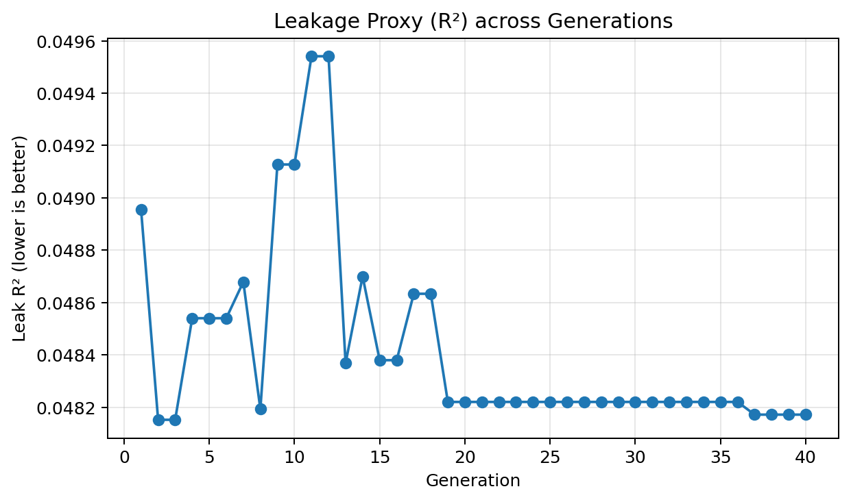
Leakage \(R^2\) across generations
We track a leakage proxy defined by the linear-probe coefficient of determination \( R^2 = 1 - \tfrac{\sum_i (x_i-\hat{x}_i)^2}{\sum_i (x_i-\bar{x})^2} \). Lower is better: a smaller \(R^2\) means transcript features explain less variance in the secret, so a linear attacker requires more data and suffers higher error.
In this run, leakage moves from 0.0490 → 0.0482. The absolute delta is intentionally modest—at this regime the probe already performs poorly—so the important signal is the shape: an early descent (easy wins), a mid-run plateau (search trades cost for diversity), and a later stabilization near a floor under the linear attacker. This behavior aligns with NSGA-II’s elitism and the self-adaptive mutation schedule.
- Downward steps indicate configurations that decorrelate transcript statistics from the secret (e.g., stronger blinding, less structured batching).
- Plateaus reflect frontier maintenance—no linear-probe gain without paying cost; see the kick plot for targeted step expansion.
- Next: if policy demands even lower leakage, keep the optimizer but upgrade the probe (kernel ridge / small MLP) to test non-linear leakage.
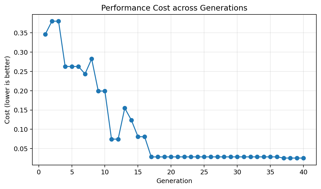
Cost across generations
The cost axis is a monotone proxy \( C(\theta)=w_t T(\theta)+w_m M(\theta)+w_o O(\theta) \). We observe a drop from 0.3463 → 0.0255 (−92.63%). The steep early descent corresponds to removing dominant overheads that also benefit leakage (dual-improvement region). The long flat tail indicates a tight frontier: further cost cuts would trade off leakage.
- Early slope = exploitation: many individuals reduce both \(L\) and \(C\).
- Tail = diversification: crowding distance preserves a spread of options to enable knee selection.
- Deployment: replace proxy with measured prover/verify wall-clock and peak memory to obtain a production S-curve.
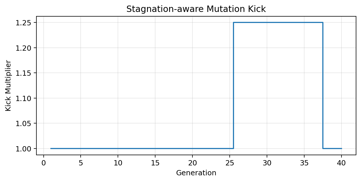
Stagnation-aware mutation kick
The kick multiplier engaged 12 time(s), peaking at 1.25. We update per-gene step sizes via \( \sigma'=\sigma\,e^{\tau_0 N(0,1)+\tau N_i(0,1)}\cdot\kappa \) and reflect at bounds. Kicks are only applied on no-improvement windows, expanding exploration just enough to escape local basins without collapsing the frontier.
Design rule: cap \(\kappa\) so that the expected one-step movement remains <10% of the parameter range; this preserves stability.
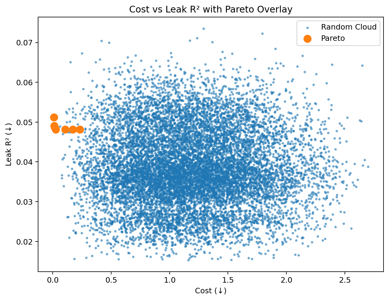
Frontier geometry and knee selection
Blue samples show explored configurations; highlighted points are non-dominated. The frontier quantifies the trade-off surface: points below-left are universally preferred. We normalize each axis and choose the knee by minimizing distance to the origin \( \operatorname*{argmin}_i\sqrt{\tilde L_i^2+\tilde C_i^2} \), producing a balanced default.
Interpretation: a convex-looking frontier indicates many mutually beneficial improvements are exhausted; a concave frontier suggests residual “free lunch” zones. Here the mixed shape implies local free-lunch pockets at low cost and a sharp shoulder near the knee.
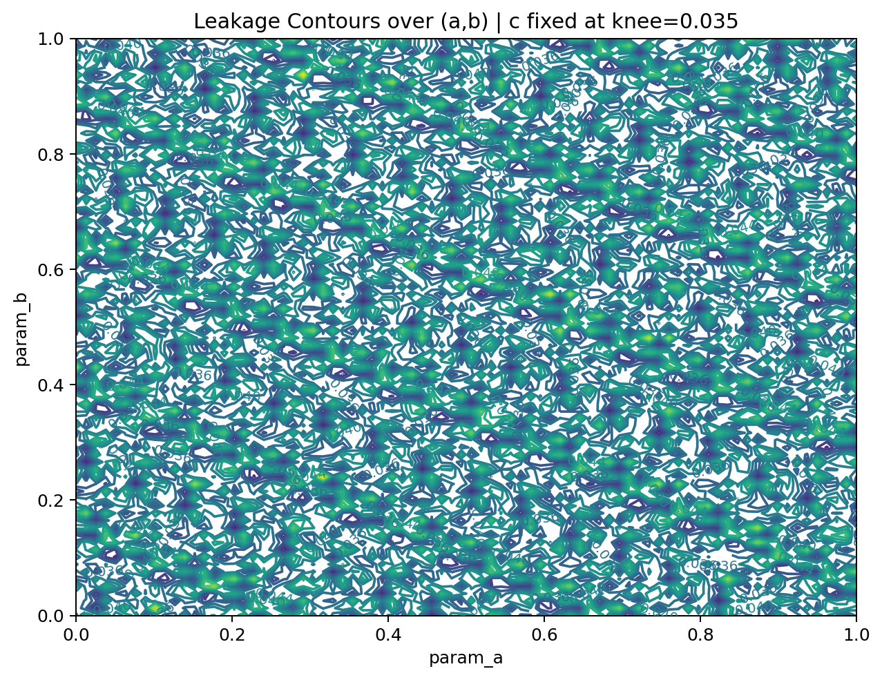
Local anisotropy (sensitivity)
Contours expose directions of unequal sensitivity. Gentle slopes mark robust directions (hyper-parameters less critical); steep slopes demand tighter control and motivate anisotropic mutation. Self-adaptation naturally takes larger steps on flatter axes and smaller steps along steep axes, improving convergence without sacrificing stability.
Operationally: lock down the steep axis with stricter bounds; allow wider auto-tuning on the flat axis.
Basins and ridges explain plateaus
The surface shows shallow basins separated by mild ridges—consistent with the plateau segments in the leakage curve. Step-size adaptation plus occasional kicks are sufficient to traverse these features; no heavy restart policy is required. If future surfaces show sharp cliffs, consider constraint softening or a two-phase schedule (global exploration → local polish).
Frontier support & knee
The frontier is supported by multiple distinct \((a,b,c)\) combinations. The knee at index 4 achieves leak 0.048172 and cost 0.025540 with \( a=0.007789,\ b=0.003807,\ c=0.034663 \). Having several near-knee neighbors is desirable operationally: it allows bounded tweaks (e.g., memory caps) without falling off the frontier.
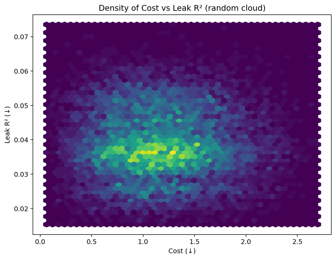
Where the search invested effort
The density cloud highlights frequently visited regions and shoulder points. Mass concentration near the shoulder indicates the optimizer repeatedly returns to balanced solutions—another signal that the knee is a stable choice.
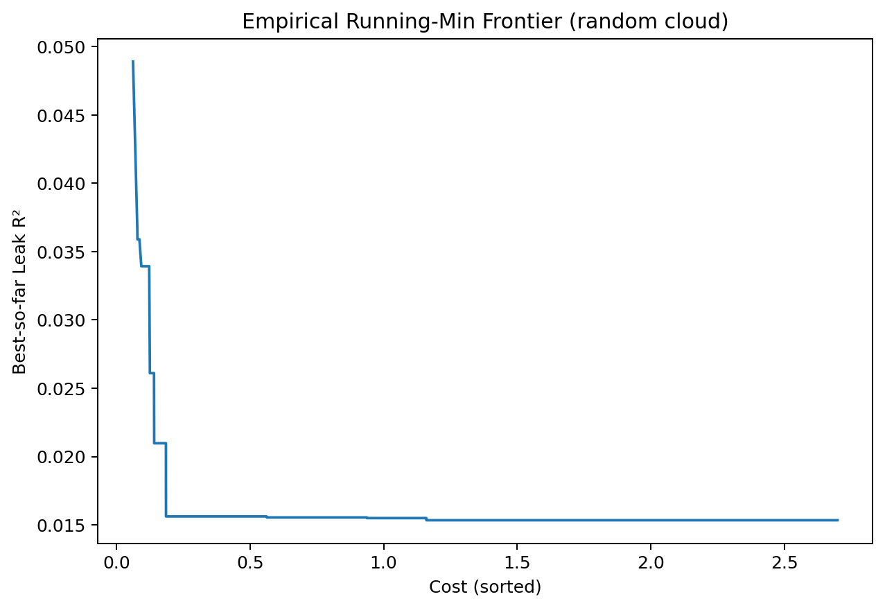
Sampling envelope sanity check
Sorting samples by cost and tracking the running minimum of leakage yields an empirical envelope that should lie above or near the true frontier. Its shape here is compatible with the Pareto overlay, suggesting consistent sampling and no major blind spots.
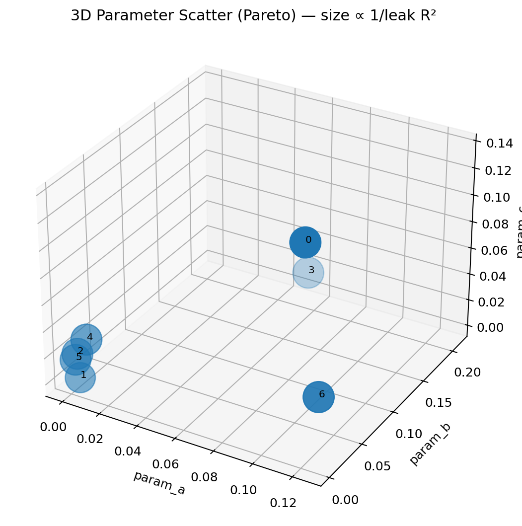
Interactive 3D
Interactive: Parameter Cloud + Pareto
How to read the 3D Parameter Cloud + Pareto
Every dot is one experiment at a parameter triple \( \theta=(a,b,c) \).
Blue points are all sampled configurations; red points are
Pareto-optimal (non-dominated) — no other configuration beats them on both leakage and cost.
Hover a point to see its measured leakR2 and cost.
Why 3D? The search space is genuinely three-parameter. In 2D projections (\(a\)–\(b\), \(a\)–\(c\), \(b\)–\(c\)) interactions get flattened and can look falsely monotone. The 3D view shows:
- Clusters of viable regions: groups of points where many \(\theta\) produce similar (leak, cost).
- Ridges/voids in parameter space: directions that almost never yield good trade-offs.
- Frontier support: whether your Pareto red points cover a broad part of the cube (healthy diversity) or sit on a thin shelf (brittle).
What to look for: rotate to check if the red Pareto set forms a bowed arc
through the cloud.
A smooth arc implies stable trade-offs; a broken or branched arc suggests multiple regimes you might want to
document as alternative presets (e.g., low-cost
vs low-leak
).
Actionable: Use the 3D scatter to set bounded ranges for each parameter: trim away volumes with no red (Pareto) presence and seed future runs with priors near the red arc.
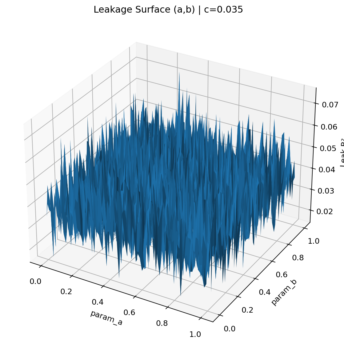
Interactive: Leakage Surface (a,b)
How to read the Interactive Leakage Surface
This is the function \(L(a,b\,|\,c^\ast)\) — leakage (vertical axis) as you vary \(a\) and \(b\) with \(c\) fixed to your knee. It’s the 3D counterpart of a contour plot: rotate to see valleys (good) and ridges (bad).
Local sensitivity. Steep regions mean small errors in \(a\) or \(b\) change leakage a lot. Flat regions are robust. Formally, the gradient \( \nabla L = \bigl[\tfrac{\partial L}{\partial a},\tfrac{\partial L}{\partial b}\bigr] \) encodes slope and the Hessian’s top eigenvector shows the most sensitive direction. Qualitatively:
- Wide, shallow basins → forgiving defaults; mutation can take larger steps.
- Narrow gullies → tight tolerances; reduce mutation step size or clamp bounds.
- Plateaus → expect optimizer stagnation unless you introduce kicks (visible in your history).
Why 3D? In 2D you can’t see joint curvature: a ridge that is gentle in \(a\) and gentle in \(b\)
can still be sharp along some diagonal combination. The surface view makes these diagonal cliffs
obvious.
Rule of thumb: pick operating points in wide basins even if they are a hair above the absolute minimum — you gain robustness to drift and hardware noise with negligible leakage penalty.
Interactive: Trajectory
How to read the Animated Knee Trajectory
Each frame plots the current knee candidate
in parameter space as the optimizer advances.
You’re seeing where in \((a,b,c)\) the balanced solution lives over generations.
- Long, smooth moves early → exploitation of easy wins, often accompanied by sharp cost drops.
- Stutters/pauses → frontier polishing; typically coincide with flat segments in the leakage curve.
- Small jumps after stalls → effect of the mutation kick; good sign you’re escaping shallow basins.
Convergence heuristic. Track the path length \( S=\sum_t \lVert \theta_{t+1}-\theta_t\rVert_2 \). When \( \lVert \theta_{t+1}-\theta_t\rVert_2 \) stays below a small threshold for several frames and your knee’s normalized distance \( \sqrt{\tilde L^2+\tilde C^2} \) no longer improves, the run has stabilized.
Why 3D? The knee can shift mainly along one parameter (say, \(c\)) while appearing stable in 2D projections. The trajectory reveals which parameter is still active, guiding which bounds to tighten and where to focus ablations.
Why 3D matters for ZK parameter tuning
ZK systems often have interacting knobs: a setting that looks safe for \(a\) at one \(b\) can leak at another. 3D views prevent false conclusions from flattened 2D slices by exposing clusters, ridges, and multiregime structure in the full \((a,b,c)\) space. Practically, this lets you (i) prune dead volumes, (ii) pick robust basins over brittle minima, and (iii) document alternate presets when the Pareto set branches.
Pareto Knee Summary
| Knee idx | Leak R² | Cost | a | b | c | Pareto size |
|---|---|---|---|---|---|---|
| 4 | 0.048172 | 0.025540 | 0.007789 | 0.003807 | 0.034663 | 7 |